BOSE-EINSTIEN DISTRIBUTION
Suppose we have a number of energy levels, labeled by index , each level having energy
  and containing a total of
  particles. Suppose each level contains
  distinct sublevels, all of which have the same energy, and which are
distinguishable. For example, two particles may have different momenta,
in which case they are distinguishable from each other, yet they can
still have the same energy. The value of associated with level is called the "degeneracy" of that energy level. Any number of bosons can occupy the same sublevel.
distinct sublevels, all of which have the same energy, and which are
distinguishable. For example, two particles may have different momenta,
in which case they are distinguishable from each other, yet they can
still have the same energy. The value of associated with level is called the "degeneracy" of that energy level. Any number of bosons can occupy the same sublevel.Let
 be the number of ways of distributing
  particles among the
  sublevels of an energy level. There is only one way of distributing particles with one sublevel, therefore
  . It is easy to see that there are
  ways of distributing particles in two sublevels which we will write as:
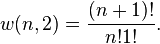 particles in three sublevels is
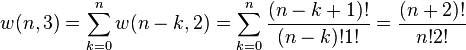
 is just a binomial coefficient (See Notes below)
 can be realized is the product of the ways that each individual energy level can be populated:
 .
.Following the same procedure used in deriving the Maxwell–Boltzmann statistics, we wish to find the set of
for which W
is maximised, subject to the constraint that there be a fixed total
number of particles, and a fixed total energy. The maxima of  and
and  occur at the value of
  and, since it is easier to accomplish mathematically, we will maximise
the latter function instead. We constrain our solution using Lagrange multipliers forming the function:
and, since it is easier to accomplish mathematically, we will maximise
the latter function instead. We constrain our solution using Lagrange multipliers forming the function: approximation and using Stirling's approximation for the factorials
  gives
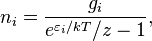
gives , and setting the result to zero and solving for , yields the Bose–Einstein population numbers:

 becomes a statement of the second law of thermodynamics at constant volume, and it follows that
  and
and  where S is the entropy, μ is the chemical potential, k is Boltzmann's constant and T is the temperature, so that finally:
A derivation of the Maxwell–Boltzmann distribution
Suppose we have a container with a huge number of very small identical particles. Although the particles are identical, we still identify them by drawing numbers on them in the way lottery balls are being labelled with numbers and even colors.All of those tiny particles are moving inside that container in all directions with great speed. Because the particles are speeding around, they do possess some energy. The Maxwell–Boltzmann distribution is a mathematical function that speaks about how many particles in the container have a certain energy.
It can be so that many particles have the same amount of energy εi. The number of particles with the same energy εi is Ni. The number of particles possessing another energy εj is Nj. In physical speech this statement is lavishly inflated into something complicated which states that those many particles Ni with the same energy amount εi, all occupy a so called "energy level" i . The concept of energy level is used to graphically/mathematically describe and analyse the properties of particles and events experienced by them. Physicists take into consideration the ways particles arrange themself and thus there is more than one way of occupying an energy level and that's the reason why the particles were tagged like lottery ball, to know the intentions of each one of them.
To begin with, let's ignore the degeneracy problem: assume that there is only one single way to put Ni particles into energy level i . What follows next is a bit of combinatorial thinking which has little to do in accurately describing the reservoir of particles.
The number of different ways of performing an ordered selection of one single object from N objects is obviously N. The number of different ways of selecting two objects from N objects, in a particular order, is thus N(N − 1) and that of selecting n objects in a particular order is seen to be N!/(N − n)!. The number of ways of selecting 2 objects from N objects without regard to order is N(N − 1) divided by the number of ways 2 objects can be ordered, which is 2!. It can be seen that the number of ways of selecting n objects from N objects without regard to order is the binomial coefficient: N!/(n!(N − n)!). If we now have a set of boxes labelled a, b, c, d, e, ..., k, then the number of ways of selecting Na objects from a total of N objects and placing them in box a, then selecting Nb objects from the remaining N − Na objects and placing them in box b, then selecting Nc objects from the remaining N − Na − Nb objects and placing them in box c, and continuing until no object is left outside is


 . Thus the number of ways W that a total of N particles can be classified into energy levels according to their energies, while each level i having gi distinct states such that the i-th level accommodates Ni particles is:
 relates the thermodynamic entropy S to the number of microstates W, where k is the Boltzmann constant. It was pointed out by Gibbs however, that the above expression for W does not yield an extensive entropy, and is therefore faulty. This problem is known as the Gibbs paradox The problem is that the particles considered by the above equation are not indistinguishable. In other words, for two particles (A and B)
in two energy sublevels the population represented by [A,B] is
considered distinct from the population [B,A] while for
indistinguishable particles, they are not. If we carry out the argument
for indistinguishable particles, we are led to the Bose-Einstein expression for W:
relates the thermodynamic entropy S to the number of microstates W, where k is the Boltzmann constant. It was pointed out by Gibbs however, that the above expression for W does not yield an extensive entropy, and is therefore faulty. This problem is known as the Gibbs paradox The problem is that the particles considered by the above equation are not indistinguishable. In other words, for two particles (A and B)
in two energy sublevels the population represented by [A,B] is
considered distinct from the population [B,A] while for
indistinguishable particles, they are not. If we carry out the argument
for indistinguishable particles, we are led to the Bose-Einstein expression for W:
 . The Maxwell-Boltzmann distribution also requires low density, implying that
  . Under these conditions, we may use Stirling's approximation for the factorial:

 for we can again use Stirlings approximation to write:
We wish to find the Ni for which the function W is maximized, while considering the constraint that there is a fixed number of particles
 and a fixed energy
 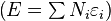 in the container. The maxima of W and ln(W) are achieved by the same values of Ni
and, since it is easier to accomplish mathematically, we will maximize
the latter function instead. We constrain our solution using Lagrange multipliers forming the function:
in the container. The maxima of W and ln(W) are achieved by the same values of Ni
and, since it is easier to accomplish mathematically, we will maximize
the latter function instead. We constrain our solution using Lagrange multipliers forming the function:
![\ln W=\ln\left[\prod\limits_{i=1}^{n}\frac{g_i^{N_i}}{N_i!}\right] \approx \sum\limits_{i=1}^n\left(N_i\ln g_i-N_i\ln N_i + N_i\right)](http://upload.wikimedia.org/wikipedia/en/math/8/5/7/85722d857301bca8c60b3b902c083190.png)


 ) we arrive to an expression for Ni:
 yields:

 is the realization that the entropy is proportional to ln W with the constant of proportionality being Boltzmann's constant. It follows immediately that β = 1 / kT and α = − μ / kT so that the populations may now be written:

Alternatively, we may use the fact that


Derivation of Fermi-Dirac Statistics
Consider a system of particles with allowed energy levelsWe impose the following hypotheses:


Given a specified
Thus,

Hypothesis 4 is valid as long as the number of energy levels, states and particles is sufficiently large. This hypothesis permits us to approximate the weighted average formula (1.5) for the (unconditional) occupancy distribution very well with the term corresponding to the most likely arrangement:
Our task now is to compute
and therefore:
To simplify the algebra to follow, instead of maximizing

We now invoke Stirling's approximation formula: for large n,
We apply this approximation:
We now maximize (1.10) subject to the constraints that

is maximized. We first locate critical points where
Note that
Letting

and thus:
for some constants
As a final remark, we often write